A data engineer, some waste-water and graph theory walk into a bar…..
Sludge 101
Right, before we delve any deeper into this there’s clearly a few questions that need answering. Whilst I imagine the majority of people could have a good stab at telling you what a data engineer does and that graph theory is something mathsy, I’m going to assume their less au fait with the lesser known world of waste water treatment, and sludge (both shown in figure 1 below).
So to quickly get people up to speed I’ve thrown up a quick Q&A, a sort of elevator pitch for sludge…
What is sludge and how does it relate to waster water? Sludge is a colloquial term for the biological matter that is removed during the treatment of waster water.
Is it important? Whilst obviously sludge will never top a water companies priority list, it is still a very important aspect of water treatment and recycling, which is essential for continuing water supplies.
What happens to it? Once treated to remove harmful bacteria, sludge is used in agriculture to help fertilise soil and crops.
Why should I care? Well as with most utilities the only way you’ll ever need to care is if the price goes up (however for water this is highly regulated) or if something goes wrong. In the latter case this could impact a water companies general operations, which you never want and is why they take it rather seriously!
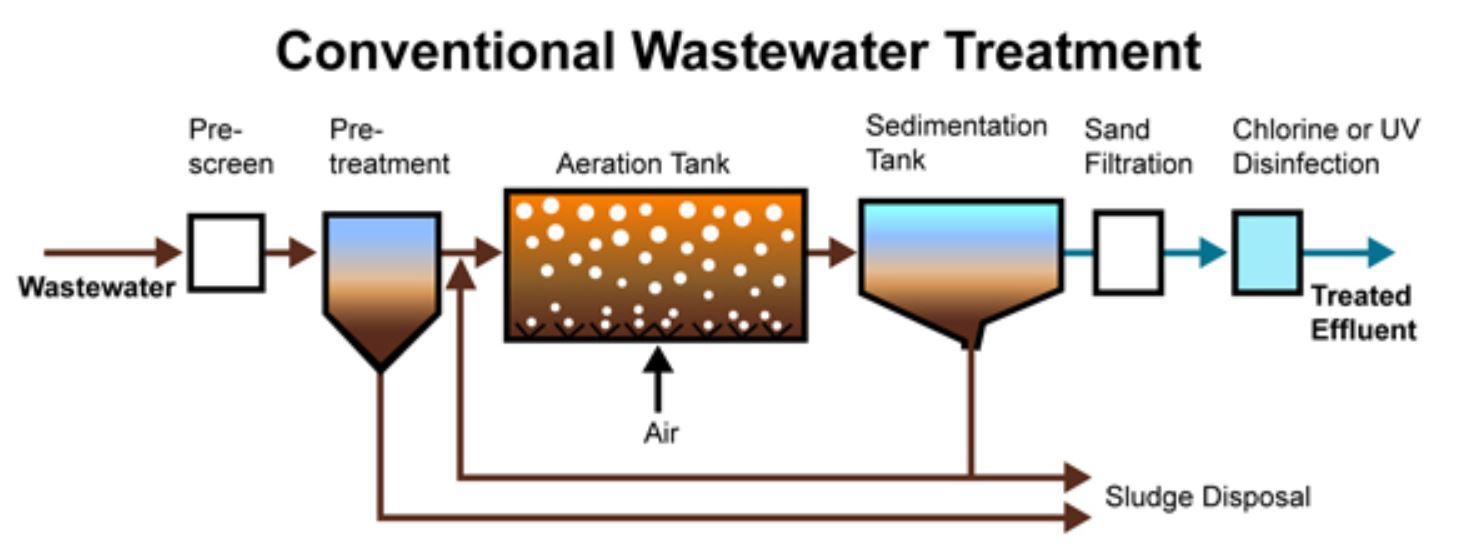
Figure 1 - The conventional waste water treament process, generating sludge
So how do you solve a problem like… Sludge?
Now you know a bit more about what sludge is, we can go into the treatment process and how this has brought about an interesting planning problem!
Once produced at a water treatment facility sludge can be handled in two key ways, it can either be thickened to one of two levels of water density or sent directly to where it it can be digested (as shown in figure 2), a process which also produces bio-gas that can be used to generate electricity. A water company will hold a number of each of these different site types, those that just produce raw, unthickened sludge, those that produce raw sludge and can thicken it to one of the two levels, or finally those that produce raw sludge and can digest it.
This collection of sites is what presents our problem, we have a number of sites each with a specialised job and an amount of sludge produced daily that requires treatment. So how do we balance the capacity of these sites and also the resources required to move the material, whilst being cost effective (since the cost to the customer is fixed over time periods, the best way for water companies to operate is internal efficiency)?
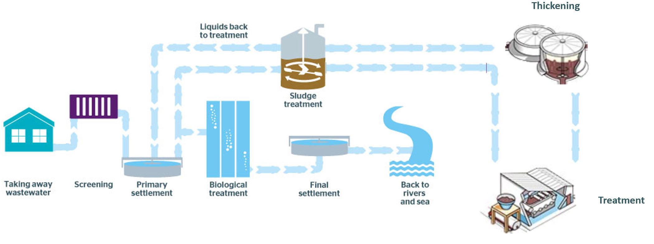
Figure 2 - The sites and movements involved in sludge production and treatment
Well on the surface it may appear there’s a simple-ish answer to this, we have a site type than can handle any type of sludge and gives us the end product whilst producing useful biogas, so problem solved! Sadly however it’s not that simple (though I doubt anyone would need help with this problem if it were…), for a few reasons, a couple of which I’ve listed below.
- Sites have limited import capacity, and calculating the movement from a large number of sites to few final processing sites can become a tough balancing act.
- Sites have a limit on vehicle access, and since unthickened sludge takes a lot of vehicles to move due to the higher water content this presents a whole world of transport pain.
- Some sites are very far from the end product site, meaning it can require a lot of drivers and vehicles to move it there, as opposed to using an intermediate thickening site.
- End sites can have varying costs based on the type of sludge their taking in, so shipping everything straight there can leave you worse off financially.
Well now that we know why it’s not that simple, how can we go about actually solving this? Well since we’ve explained the waste-water involvement and the data engineer hasn’t got enough fingers to work it out for ~600 treatment sites we’re only left with graph theory from the rather leading section title! So I guess I should probably introduce that, and then we can get cracking on the actual problem!
Not wanting to be too graphic….
First off, I’m going to throw in the disclaimer that I’m a novice mathematician at best, with my knowledge mostly centered around statistics. As such this is going to be a fairly basic, but helpful, overview of the topic, therefore if you feel like you know enough already I’d jump into the next section looking at how the networks were actually designed.
Now that’s over with, it’s worth mentioning that whilst graphs and graph theory share a fundamental element that they are structures utilised to understand the connectivity between data, they are not the same thing. Graph theory is a branch of maths that utilises objects made up of nodes (the related items, such as people in an online community) and edges (the connections between nodes), with an example shown below in figure 3. These graphs can be built up into different forms, with edges taking on various aspects such as a measure of connectivity, capacity, cost or similarity, that are then used to solve various problems such as how connected are two individuals in a social network, or how can we cluster two groups of genes based on how they interact with each other. A final key aspects of graphs, at least from the point of this work, is that they can be undirected, flow can move both ways across an edge, or directed, flow is unidirectional across an edge.
In our case, we can build up the sites as nodes in a directed graph, with edges containing information on capacity and costs, allowing us to utilise a network based algorithm to solve for the production in the network at the minimum cost based on the information provided in the edges.
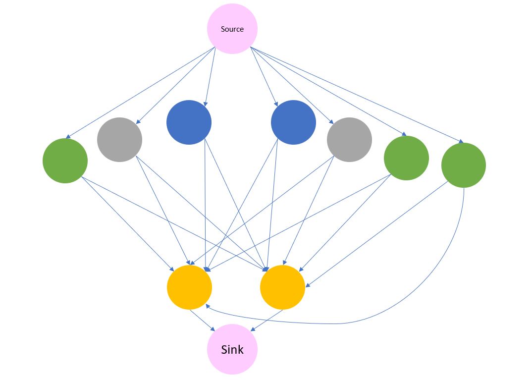
Figure 3 - An example graph made up of a collection of nodes (circles) and edges (lines)
Expanding our network….
So now we have the component concepts down how do we go about creating a network (or graph) of our sites and solving our problem? Well for ease of visualisation I’ll showcase it using a toy example of around 6 sites, which still incorporates all our required site types, but I’ll also explain a couple of the important elements that are needed when scaling up to a full set of sites.
Starting simple, below is the code to build a 6 site network (which is alos shown in figure 4), with connections moving down through the site types, i.e raw sludge producing sites (type A) can connect to any site except their own type, first thickener sites (type B) can connect to further thickeners (type C) and final sites (type D), etc, etc. In the real network this is controlled by giving sites numeric ranks based on their type, which can then be used to filter connections, allowing a site type change in the input data to subsequently be deployed in the network. This gives some flexibility if say the equipment malfunctions at a site and can no longer perform its defined function.
# a very useful network analysis library
import networkx as nx

# create an empty, directed graph
G = nx.DiGraph()

# add nodes from list, with associated production (-) / capacity (+)
G.add_nodes_from([("A-1", {"demand" : -3}), ("A-2", {"demand" : -3}), ("B-1", {"demand" : -3}),
                  ("B-2", {"demand" : -3}), ("C-1", {"demand" : -3}), ("D-1", {"demand" : 15})])

# add edges with capacities and weight (cost)
G.add_edges_from([("A-1", "B-1", {'capacity': 3, 'weight': 4}),
                   ("A-1", "B-2", {'capacity': 5, 'weight': 6}),
                   ("A-2", "B-1", {'capacity': 3, 'weight': -3}),
                   ("A-2", "B-2", {'capacity': 5, 'weight': 1}),
                   ("A-1", "C-1", {'capacity': 2,'weight': 9}),
                   ("A-1", "D-1", {'capacity': 15, 'weight': 5}),
                   ("A-2", "C-1", {'capacity': 2, 'weight': 13}),
                   ("A-2", "D-1", {'capacity': 15, 'weight': 0}),
                   ("B-1", "C-1", {'capacity': 2, 'weight': 2}),
                   ("B-2", "C-1", {'capacity': 2, 'weight': 1}),
                   ("B-1", "D-1", {'capacity': 15,'weight': 8}),
                   ("B-2", "D-1", {'capacity': 15, 'weight': 6}),
                   ("C-1", "D-1", {'capacity': 15, 'weight': 6})])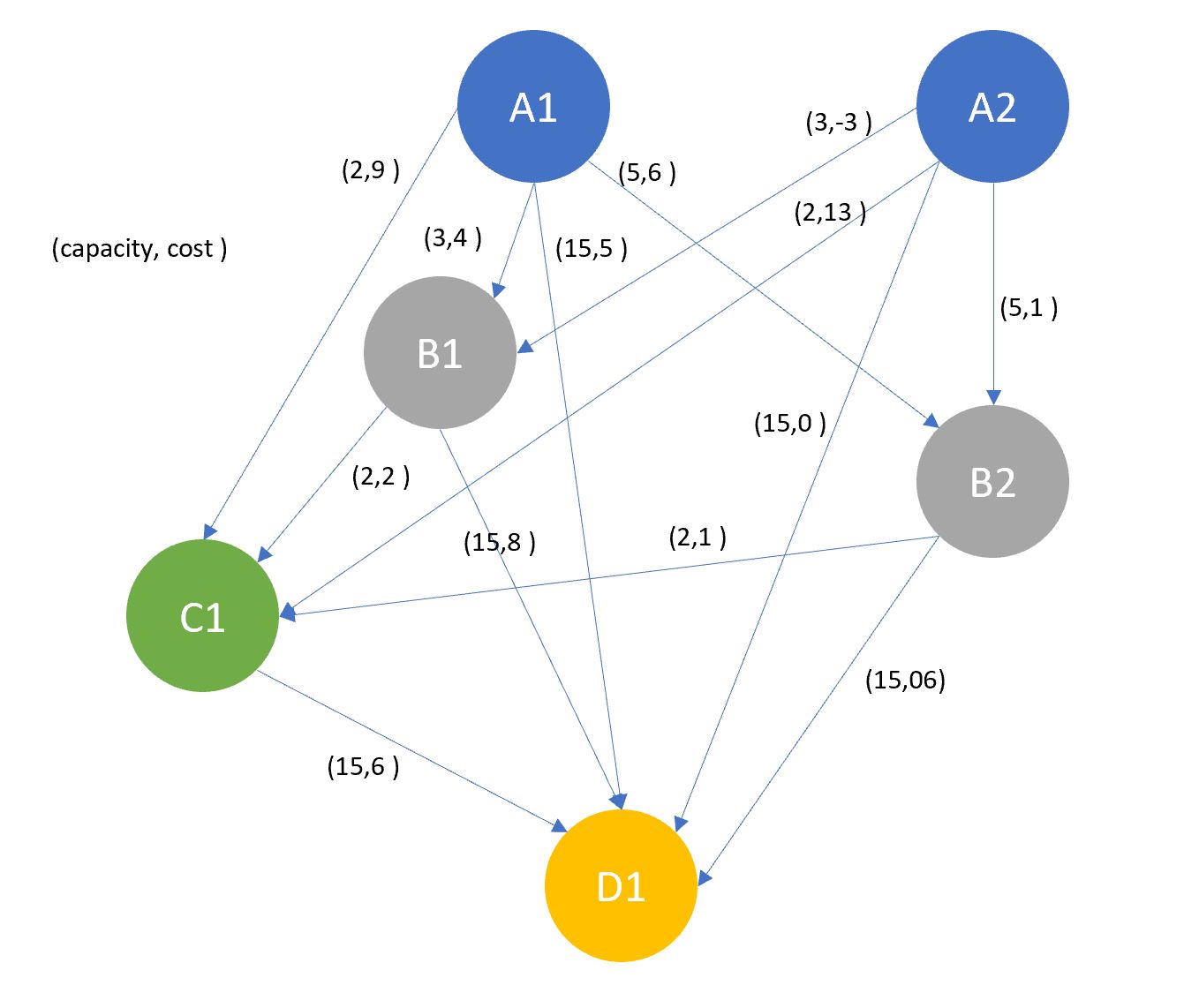
Figure 4 - A representation of the network produced in the code above
Okay, so now we have a representative network we can go ahead and solve it right? Well not just yet actually, there’s a couple of things we need to do to make it truly representative, one on the actual structure of the network and a few in the data that feeds it (though I’ll just discuss these rather than writing out the associated data tables!)
Starting with the more data centric adjustments, which fall into two main categories, there is a need to adjust capacities based on indigenous production and also alter costs to highlight the distance between sites, why these are required is explained below.
The first is required due to a couple of processes that occur at the final site, electricity generation and the method by which the sludge is treated. Both of these processes have capacity thresholds and as such must be adjusted based on the indigenous production fo the site (as this will be treated before any imports). This can be performed fairly easily when building cost tables, though corrections will need to be made if indigenous production is higher than the max threshold of either process!
The second is important due to the resource cost of moving material long distances, especially material with high liquid content, as mentioned previously. Now this may well be reflected by a distance based costing approach, but if third party contractors are used this may be banded, losing some of the detail. This can be amended by developing a cost function based on distance, and then applying it to the banded transport costs.
Moving on to the structural element, the main issue we have with the current set up is that it can’t control for a nodes capacity, as this is designated on the edges. As an example, node C above may have a capacity of 3, which is reflected in each of the edges, however as there is no capacity measure on the node this may allow the network to send more than 3 units to said node. We can remove this problem by using “gate-nodes”, as shown in figure 5, that sit in front of those that can receive multiple inputs, controlling the total flow towards it. In order to do this we’ll need to rebuild our above network, with a few additional elements.
G2 = nx.DiGraph()

# add nodes, including those acting as gates
G2.add_nodes_from([("A-1", {"demand" : -3}), ("A-2", {"demand" : -3}), ("B-1", {"demand" : -3}), ("B-1-G", {"demand" : 0}),
                  ("B-2", {"demand" : -3}), ("B-2-G", {"demand" : 0}), ("C-1", {"demand" : -3}), ("C-1-G", {"demand" : 0}),
                  ("D-1", {"demand" : 15}), ("D-1-G", {"demand" : 0})])

# add edges with capacities and weight (cost)
G2.add_edges_from([("A-1", "B-1-G", {'capacity': 3, 'weight': 4}),
                   ("A-1", "B-2-G", {'capacity': 5, 'weight': 6}),
                   ("A-2", "B-1-G", {'capacity': 3, 'weight': -3}),
                   ("A-2", "B-2-G", {'capacity': 5, 'weight': 1}),
                   ("A-1", "C-1-G", {'capacity': 2,'weight': 9}),
                   ("A-1", "D-1-G", {'capacity': 15, 'weight': 5}),
                   ("A-2", "C-1-G", {'capacity': 2, 'weight': 13}),
                   ("A-2", "D-1-G", {'capacity': 15, 'weight': 0}),
                   ("B-1", "C-1-G", {'capacity': 2, 'weight': 2}),
                   ("B-2", "C-1-G", {'capacity': 2, 'weight': 1}),
                   ("B-1", "D-1-G", {'capacity': 15,'weight': 8}),
                   ("B-2", "D-1-G", {'capacity': 15, 'weight': 6}),
                   ("C-1", "D-1-G", {'capacity': 15, 'weight': 6}),
                   ("B-1-G", "B-1", {'capacity': 3, 'weight': 6}),
                   ("B-2-G", "B-2", {'capacity': 5, 'weight': 6}),
                   ("C-1-G", "C-1", {'capacity': 2, 'weight': 6}),
                   ("D-1-G", "D-1", {'capacity': 15, 'weight': 6})])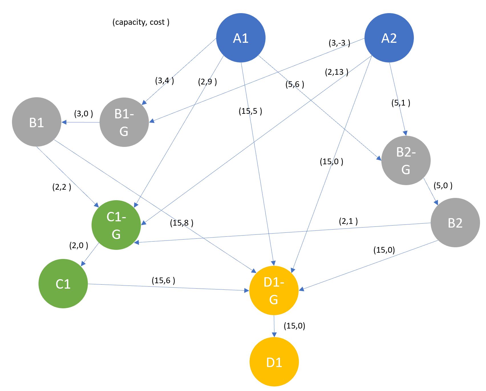
Figure 5 - A representation of the above network, including gate nodes
Now that we have a complete network we can utilise an algorithm in order to solve the problem, at hand, ie dealing with the production in the system (designated by the -ve demand in the nodes above) through the available capacity and at the lowest associated cost. There are a number of algorithms utilised to deal with flow in graph theory, such as Edmonds-Karp and max-flow, however the most appropriate for this scenario is a linear solving method known as the network simplex model. In essence, this solver works by moving units through the network from production sites to sink sites for the lowest possible cost, altering movements where a cheaper solution can be found.
flowCost, flowDict = nx.network_simplex(G2)## 165## {'A-1': {'B-1-G': 0, 'B-2-G': 0, 'C-1-G': 0, 'D-1-G': 3}, 'A-2': {'B-1-G': 0, 'B-2-G': 0, 'C-1-G': 0, 'D-1-G': 3}, 'B-1': {'C-1-G': 0, 'D-1-G': 3}, 'B-1-G': {'B-1': 0}, 'B-2': {'C-1-G': 0, 'D-1-G': 3}, 'B-2-G': {'B-2': 0}, 'C-1': {'D-1-G': 3}, 'C-1-G': {'C-1': 0}, 'D-1': {}, 'D-1-G': {'D-1': 15}}Shown above are the outputs of this method, namely a total cost of the optimal solution and also the node to node flow, which can then be used to build any associated outputs that may be required. These would likely encompass details such as the amount of biogas generated, associated transport costs and distances, chemical requirements and other costs that may arise in the process. Such outputs could then be summarised to provide different detail levels required by different people, ie high detail for those involved in detailed planning and lower detail for those solely interested in cost and resource implications at the top level. Outputs at levels similar to what is discussed above is shown in figure 6.
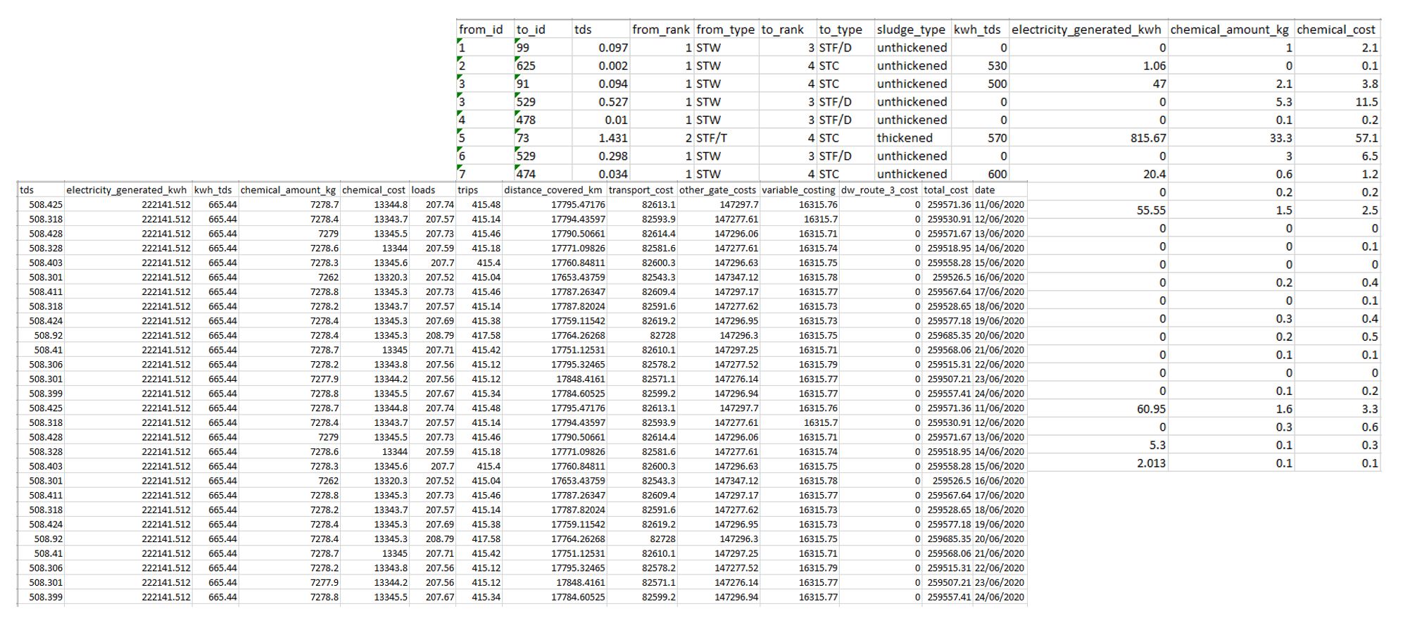
Figure 6 - Example outsputs at the sludge movement and aggregated run level
So no more sludge problems?
Whilst I can hope this short intro is enlightening and somewhat entertaining, I can’t say that its definitively solved the problem. For one there’s a few elements that I’ve not incorporated just to keep the article from expanding into a waste-water based mess…
This includes aspects like additional gate nodes for dealing with the amount of high and low liquid density loads a site can deal with and the variable capacity aspects derived from biogas generation and other elements (ie the production of biogas lowers the cost of treatment up to a certain threshold, so at least 2 costs are required based on a nodes capacity).
Then there’s how the input and output data is manipulated to either adjust the input data, for things calculating the variable cost implications from biogas generation, or build up the output data, to give the required detail for elements that feed into the process such as chemical usage.
Finally there’s how to actually build and deploy the above as a solution, it’s no help to anyone if it’s just sitting on a laptop waiting for someone to run it. It needs to be built up into a maintainable, scalable application, which most likely relies on utilising some open source software (we’ve already made a start by using Python to create and run the graph) and getting in running either on premise or in the cloud where it can be used effectively!
(I will however point out that it would be somewhat remiss of me to bring up these questions if I hadn’t gone through them myself whilst attempting to solve this problem)