Intro
This short post is an attempt to compare two commonly used clustering methods, hierarchical and k means, utilising a wheat seeds data set from the online machine learning repository
Analysis
First thing as always is to load packages, with a mix of cleaning, clustering and graphing packages for this analysis.
library(tidyverse)
library(clustree)
library(cluster)
library(scales)
library(gridExtra)
library(devtools)
library(gganimate)
Now its time to load in the data set and tidy it up. This involves setting a random seed for the later splitting of the data, assigning proper column names, rounding the values and removing any NAs
set.seed(101)

seeds <- read.delim("seeds_dataset.txt",
                   sep = "\t", header = FALSE)

colnames(seeds) <- c('area','perimeter','compactness','length_of_kernel',
                     'width_of_kernal','asymmetry_coefficient','length_of_kernel_groove',
                     'type_of_seed')

seeds$type_of_seed <- round(seeds$type_of_seed)

seeds <- drop_na(seeds)
Now that the data is clean it’s time to remove the label column and scale the data so that each value column has an equal SD and mean, to prevent different units impacting the analysis, IE a 2 foot change in height shouldn’t have the same impact as a 2kg change in weight.
seed_label <- select(seeds, type_of_seed)

seed_cluster <- select(seeds, -type_of_seed)

seed_cluster_scaled <- as_tibble(scale(seed_cluster))
Now the data is ready it’s time to test the first methodology, hierarchical clustering, which in essence places each point in its own cluster and then combines them until you converge on a single cluster, using a chosen distance metric (Max, Min, Mean or Centroid). The first part of this process was creating two functions, one to run the clustering and one to plot it, as I wanted to run a few distance types and compare the results.
heir_func <- function(x,y){
  dist(x, method  = "euclidean") %>%
    hclust(method = y)
}

plot_heir <- function(x,y){
  plot(x, hang = -1, cex = 0.4, main = paste("Seed clusters using",y,"linkage") )
}
Once the functions are set I can run each analysis and plot the results, as shown below.
seed_av <- heir_func(seed_cluster_scaled, "average")

plot_heir(seed_av,y = "average")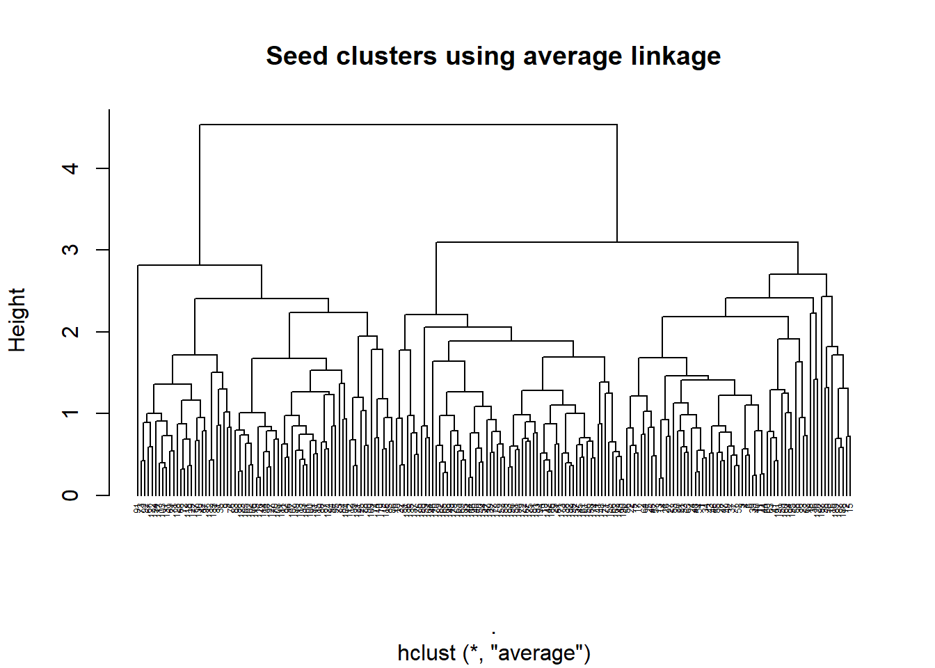
seed_comp <- heir_func(seed_cluster_scaled, "complete")

plot_heir(seed_comp, "complete")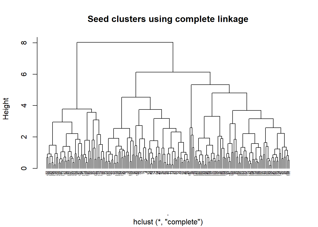
seed_cent <- heir_func(seed_cluster_scaled, "centroid")

plot_heir(seed_cent, "centroid")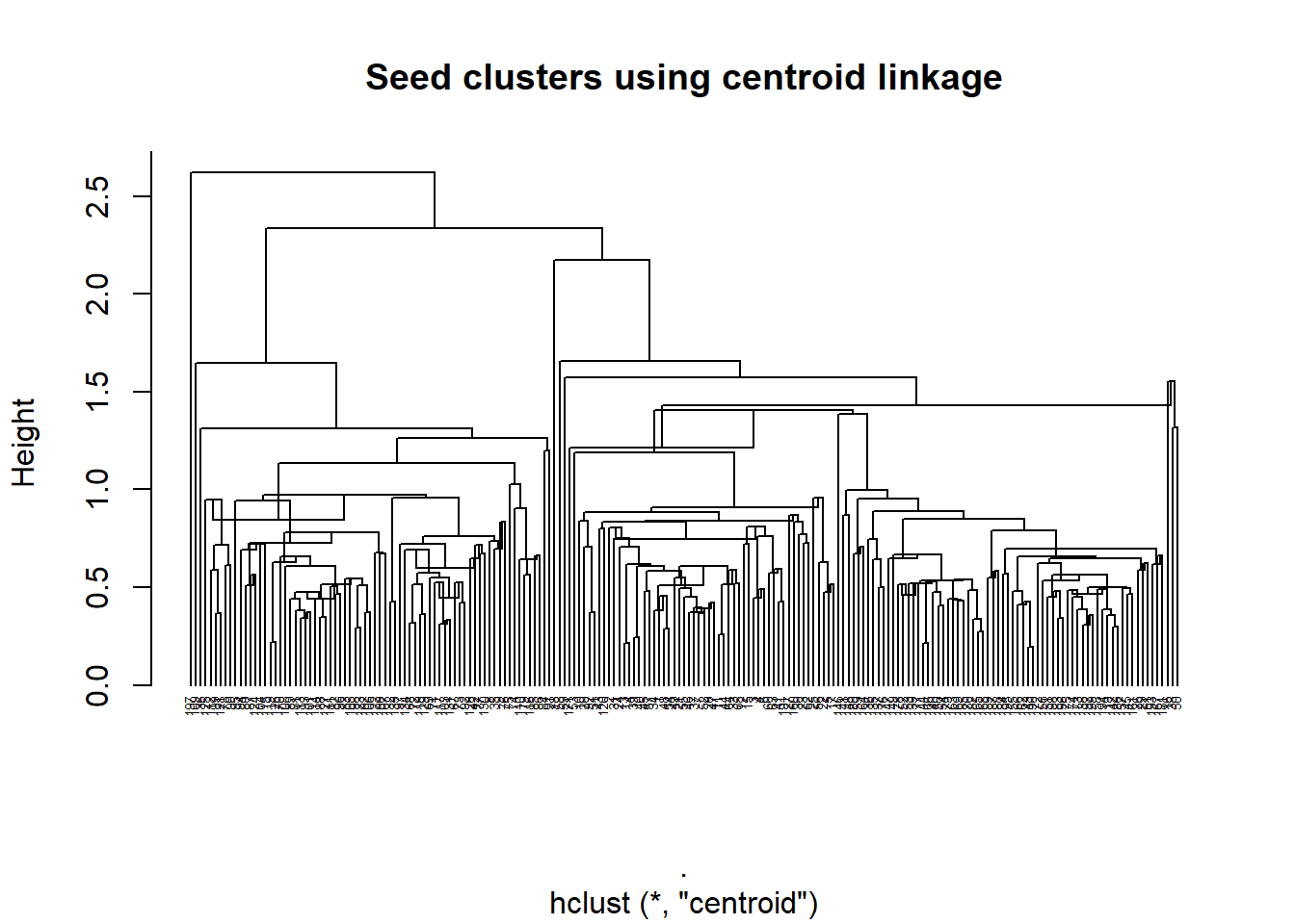
Now that we have a few clusters based on difference distances, we can plot them in an animated chart using gganimate and compare them to the actual clusters.
seeds_h_clust <- mutate(seeds, Av_clus = cutree(seed_av, k = 3),
                        Comp_clus = cutree(seed_comp, k = 3),
                        Cent_clus = cutree(seed_cent, k = 3)) %>%
  select(c(1:2, 8:11)) %>%
  mutate_at(vars(3:6), funs(as.factor)) %>%
  rename(Actual = type_of_seed, Average = Av_clus, Complete = Comp_clus, Centroid = Cent_clus) %>%
  gather(key = "Method", value = "Cluster", c(3:6)) %>%
  mutate(Method = factor(Method, levels = c("Actual", "Average", "Complete", "Centroid")))
## Warning: funs() is soft deprecated as of dplyr 0.8.0
## Please use a list of either functions or lambdas:
##
## # Simple named list:
## list(mean = mean, median = median)
##
## # Auto named with `tibble::lst()`:
## tibble::lst(mean, median)
##
## # Using lambdas
## list(~ mean(., trim = .2), ~ median(., na.rm = TRUE))
## This warning is displayed once per session.animated_clust <- ggplot(seeds_h_clust, aes(area, perimeter, col = Cluster)) +
geom_point(alpha = 0.6) +
theme_minimal() +
labs(x = "Seed Area",
y = "Seed perimeter",
col = "Type of seed",
title = paste("Heirarchical clustering using the {closest_state} linkage")) +
transition_states(Method, transition_length = 4, state_length = 3)Also just to help distinguish between them all, a static plot of the three test clusters and the real clusters was produced, using a function again to help with the repetition. This showed that…
clust_plot_func <- function(x, y, z){
  y <- enquo(y)
  h_clust_plot_true <- seeds_h_clust %>%
    filter(Method == x) %>%
    ggplot(aes(area, perimeter, col = !!y)) +
    geom_point(alpha = 0.6) +
    theme_minimal() +
    labs(x = "Seed Area", y = "Seed perimeter", col = "Type of seed", title = paste("Heirarchical clustering using the", z, "linkage"))
}

h_clust_plot_true <- clust_plot_func("Actual", Cluster, "Actual") +
  theme(legend.position = "none",
        axis.title.x=element_blank(),
        axis.text.x=element_blank(),
        axis.ticks.x=element_blank())


h_clust_plot_av <- clust_plot_func("Average", Cluster, "Average") +
  theme(axis.title.x=element_blank(),
        axis.text.x=element_blank(),
        axis.ticks.x=element_blank(),
        axis.title.y=element_blank(),
        axis.text.y=element_blank(),
        axis.ticks.y=element_blank())

h_clust_plot_comp <- clust_plot_func("Complete", Cluster, "Complete") +
  theme(legend.position = "none")

h_clust_plot_cent <- clust_plot_func("Centroid", Cluster, "Centroid") +
  theme(axis.title.y=element_blank(),
        axis.text.y=element_blank(),
        axis.ticks.y=element_blank())

grid.arrange(h_clust_plot_true, h_clust_plot_av, h_clust_plot_comp, h_clust_plot_cent, nrow = 2)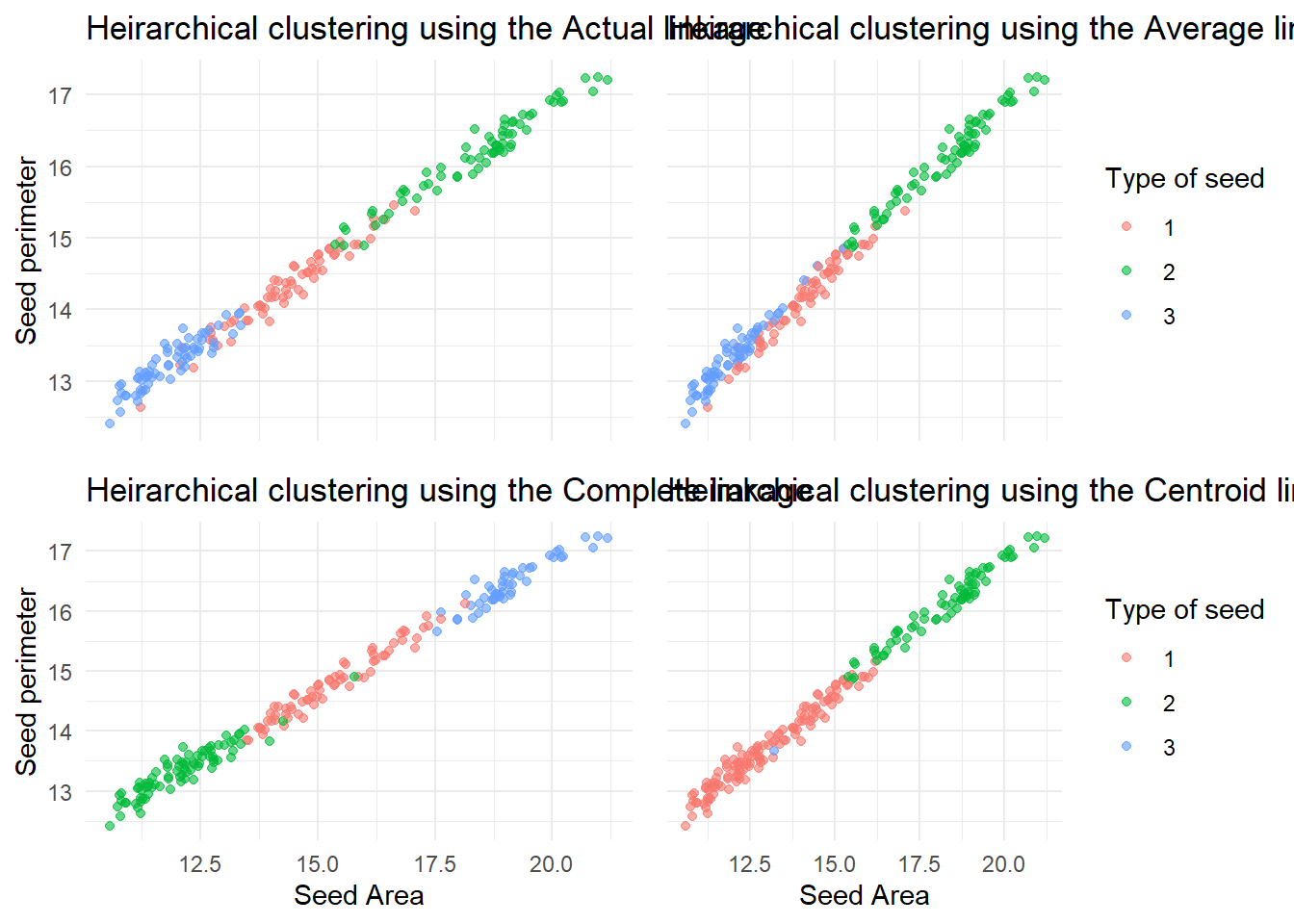
Next I moved on to K means clustering, which involves the production of k clusters through randomly assigning a start and adding new points based on a distance. This involves using the same scaled and cleaned data set from before, and specifying a few parameters for the algorithm, such as centers (how many clusters to form) and nstart(how many starts with a random new centroid)
seed_k_means <- kmeans(seed_cluster_scaled,centers = 3, nstart = 10)

clusplot(seed_cluster_scaled, seed_k_means$cluster,
                         color = T, shade  = F, lines = 0, label = 1,
                         main = "Three cluster K means analysis")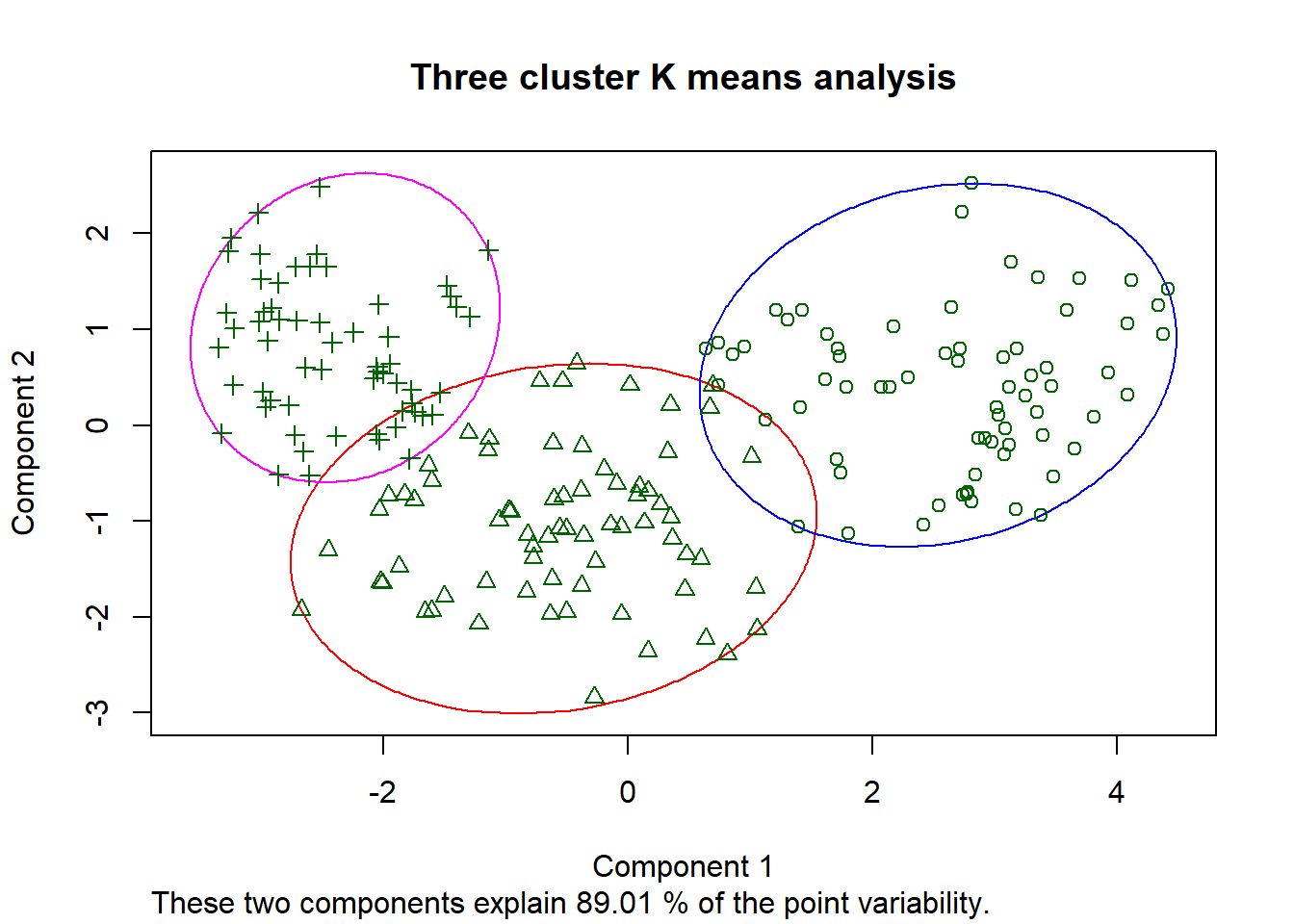
Now that we have our clusters, a more recent visualisation have been made showing how the data divides via a tree. To produce this I made a function to divide the data based on 1, 2 or 3 clusters, joined the cluster data and plotted it using the clustree package, which gives a nice visual regarding the split of the data.
clus_tree_ext <- function(x,y){
  kmeans(x,y, nstart = 10) %>%
    pluck(1) %>%
    as_tibble()
}

one_k <- clus_tree_ext(seed_cluster_scaled, 1)
## Warning: Calling `as_tibble()` on a vector is discouraged, because the behavior is likely to change in the future. Use `tibble::enframe(name = NULL)` instead.
## This warning is displayed once per session.two_k <- clus_tree_ext(seed_cluster_scaled, 2)
three_k <- clus_tree_ext(seed_cluster_scaled, 3)
seeds_k_clust <- bind_cols(one_k, two_k, three_k) %>%
rename(K1 = value, K2 = value1, K3 = value2)
clustree(seeds_k_clust, prefix = "K", layout = "sugiyama")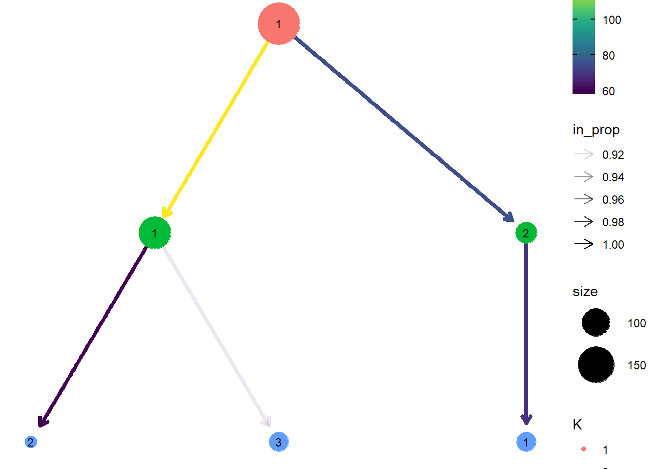
So that’s the end of this exploration on clustering, hopefully you’ve enjoyed it as much as I did researching it!