I’ve never been a huge reader, though when I do tend to get into a book it’s usually part of a larger series (ASOIAF, Harry Potter, LoTR etc). By far my favorite series of books belongs to the collection know as discworld novels, written by Sir Terry Pratchett. Between 1983 and 2015 he wrote 41 novels all surrounding a single universe, where a giant tortoise holding up a disc shaped world roamed the sky’s. Within these novels there are a range of story arcs, however my heart and soul favorite can only be given to those relating to Sam Vimes, a misanthropic, sarcastic copper that just wants to see the world in the right place.
As such, I decided to take some inspiration from two tutorials, the first relating to structural topic models (https://juliasilge.com/blog/sherlock-holmes-stm/) and the second a full text analysis of the GoT novels (https://api.rpubs.com/julheimer/got)
So, as always the first thing to do is load the packages I’ll need, with plyr and the tidyverse for general cleaning, tidytext, stm, quanteda, tm, reticulate and cleanNLP to deal with the text elements and analysis and pdftools / readtext to read in the books.
library(plyr)
library(tidyverse)
library(pdftools)
library(RColorBrewer)
library(tidytext)
library(readtext)
library(stm)
library(quanteda)
library(reticulate)
library(cleanNLP)
library(tm)
Now that we have our packages we need some data, which came from either a PDF or word document of the books. Since there was going to be a lot of repetition I designated two functions for either pdf or text extraction, which just read in the text, collapsed it and then unnested it into sentences.
PDF_extraction <- function(a){
  pdf_text(a) %>%
    paste(.,collapse = "") %>%
    tibble(text = .) %>%
    unnest_tokens(sentence, text, token = "sentences")
    }

WRD_extraction <- function(x){
  readtext(x) %>%
    unnest_tokens(sentence, text, "sentences") %>%
                    select(-1)
}
GG <- WRD_extraction("D08 - Guards! Guards!.doc")
MAA <- WRD_extraction("Men at arms.docx")
FOC <- WRD_extraction("Feet of clay.docx")
J <- WRD_extraction("Jingo.docx")
FE <- WRD_extraction("The Fifth Elephant.docx")
NW <- PDF_extraction("Night Watch.pdf")
THUD <- PDF_extraction("Pratchett_Terry-Discworld_34-Thud-Pratchett_Terry.pdf")
SNUFF <- PDF_extraction("Snuff - Terry Pratchett.pdf")Now that we have all then books split into sentences, it’s time to clean up the text and bind all the books into a single data frame. The cleaning simply involved removing the unrequired lines from each data frame and adding in a row number column as a proxy for sentence number. Once clean they were then bound together, and an reordering applied to the titles based on the order of the books.
Clean_func <- function(a,b,c){
  a %>%
    slice(b) %>%
    mutate(Book = c,
             Sentence_number = row_number())
  }

GG_DF <- Clean_func(GG, 8:10044, "Guards! Guards!")
MAA_DF<- Clean_func(MAA, 1:11113, "Men At Arms")
FOC_DF<- Clean_func(FOC, 2:10567, "Feet Of Clay")
J_DF<- Clean_func(J, 1:11360, "Jingo")
FE_DF<- Clean_func(FE, 2:11267, "Fifth Elephant")
NW_DF<- Clean_func(NW, 2:11619, "Night Watch")
THUD_DF<- Clean_func(THUD, 2:11195, "Thud")
SNUFF_DF<- Clean_func(SNUFF, 10:8072, "Snuff")


Watch_levels <- c("Guards! Guards!",
                 "Men At Arms",
                 "Feet Of Clay",
                 "Jingo",
                 "Fifth Elephant",
                 "Night Watch",
                 "Thud",
                 "Snuff")

Watch_books <- bind_rows(GG_DF, MAA_DF, FOC_DF, J_DF, FE_DF, NW_DF, THUD_DF, SNUFF_DF) %>%
  mutate(Book = factor(Book, levels = Watch_levels))
Now the data is clean and in one place, a logical starting place is a sentiment analysis of each book, using the AFINN word library, due to a better link with novels. Once the sentiments were calculated the words / scores could be counted and used to produce a ratio, which was then plotted for each sentence per novel for each dictionary, showing the positive / negative shift over the course of each book.
From the below figure you can see that sentiment varies over the timeline of each book (as you would expect) with some seeming overall a bit more cheerful than other, for example comparing Men At Arms to Snuff. This makes sense as Snuff is mostly tasked with dissecting the persecution of the goblin race.
afinn <- tidytext::get_sentiments("afinn")

watch_books_AFINN <- Watch_books %>%
  unnest_tokens(word, sentence, token = "words") %>%
  inner_join(afinn) %>%
  group_by(Book, Sentence_number) %>%
  summarise(Sentiment_score = sum(value))


watch_books_AFINN %>%
  ggplot(aes(x = Sentence_number, y = Sentiment_score, fill = Book)) +
  geom_bar(stat = "identity", show.legend = F) +
  scale_color_viridis_c() +
  facet_wrap(~Book, ncol = 3, scales = "free_x") +
  theme_minimal() +
  labs(title = "Sentiment over the Night Watch history", y = "sentiment", x = "Sentence number") +
  theme(strip.text = element_text(face = "italic")) +
  theme(panel.grid.minor = element_blank())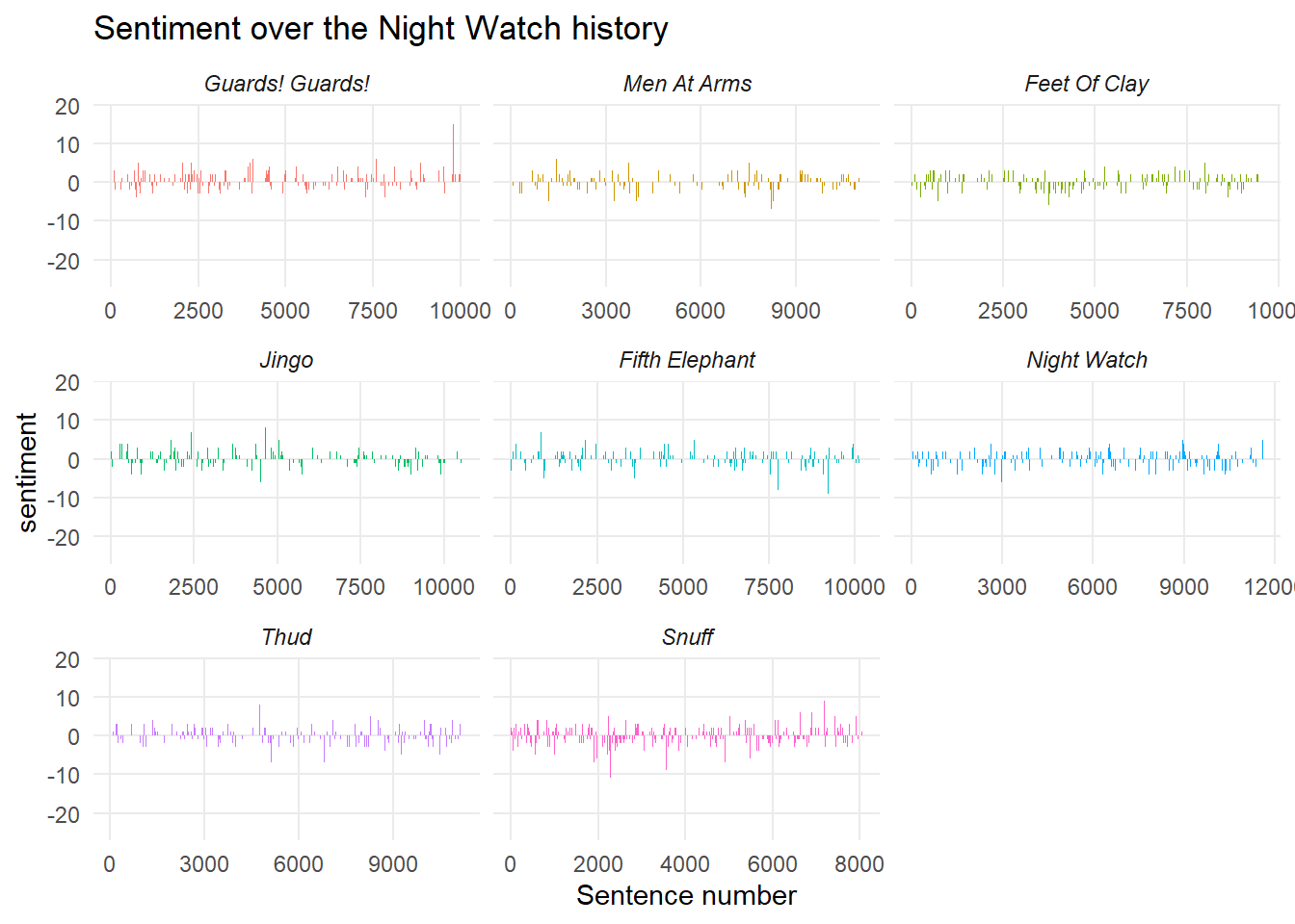
In addition to looking at each book sentence by sentence, the overall sentiment of each book was calculated and tracked across the progression of the books. This shows a somewhat different picture compared to tracking each sentence, with Men At Arms showing a lower score (thus more negative) in comparison to Snuff and Thud hitting rock bottom (likely due to all the war threats and death!)
afinn_sent_summary <- watch_books_AFINN %>%
  group_by(Book) %>%
  summarise(Overall_sentiment = sum(Sentiment_score))

afinn_sent_summary %>%
  ggplot(aes(x = Book, y = Overall_sentiment, fill= Book, group = 1)) +
  geom_line(show.legend = F, col = "red",lineend = "round", linejoin = "round", size = 1) +
  geom_point(show.legend = F, col = "orange") +
  theme_classic() +
  labs(title = "Overall sentiment score across the Night Watch books", x = "Book", y = "Overall sentiment score") +
  scale_color_brewer()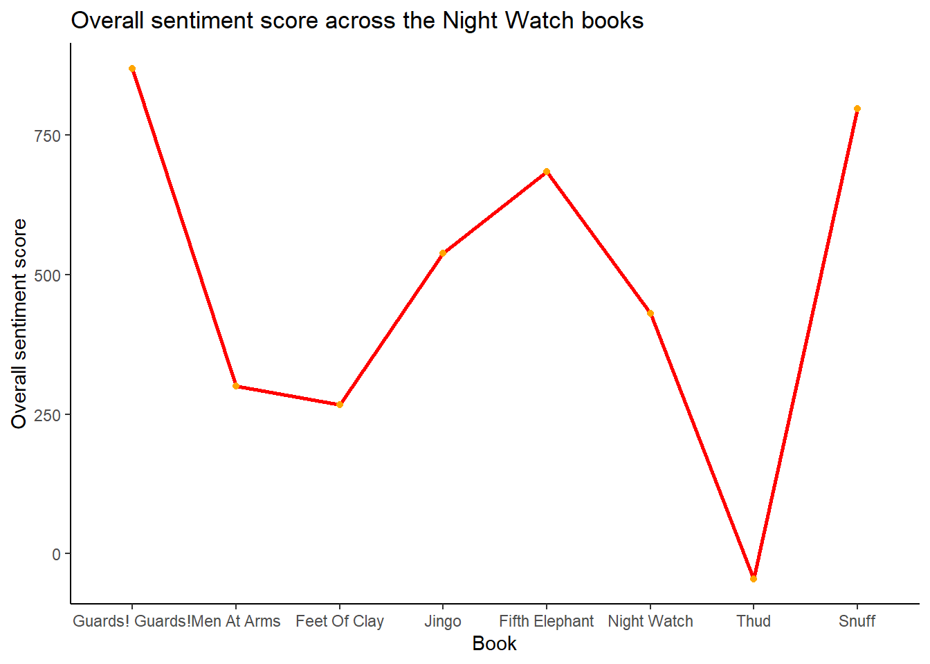
Another interesting aspect of text analysis, stole from Julia Silges wonderful blog(https://juliasilge.com/blog/gender-pronouns/) is that of gendered bigrams, IE what words are associated with he / she most commonly. So in order to do this the text had to be split into bigrams, stop words removed from each side and then put back together for counting / plotting. This was conducted for both bigrams in general and those associated with he / she.
This analysis showed that, generally, the most common bigrams were full names (such as Sam Vimes or Lord Vetinari). However, there were some interesting in book findings, such as mhm mhm within the Fifth Elephant (a phase often muttered by Inigo Skinner) and po lees within Snuff (a phrase spoken by the goblins to mean police). With regards t the gendered aspect, in general male bigrams were far more prevalent, though there was little to speak for differences in terms of actions as they mostly related to speaking / thinking.
Watch_books_bigrams <- Watch_books %>%
  unnest_tokens(bigram, sentence, token = "ngrams", n = 2) %>%
  separate(bigram, c("word1", "word2"), sep = " ") %>%
  filter(!word1 %in% stop_words$word,
         word1 != "NA",
         !word2 %in% stop_words$word,
         word2 != "NA") %>%
  count(Book, word1, word2, sort = T) %>%
  unite(Bigram, word1, word2, sep = " ") %>%
  slice(-1) %>%
  group_by(Book) %>%
  top_n(10) %>%
  arrange(Book, desc(n))

Watch_books_bigrams %>%
  ggplot(aes(x = reorder(Bigram,n), y = n, fill = Book)) +
  geom_col(show.legend = F) +
  coord_flip() +
  facet_wrap(~Book, nrow = 3, scales = "free_y") +
  theme_minimal() +
  labs(title = "Top ten bigrams in the Night Watch series",
       x = "Bigram",
       y = "Frequency") +
  scale_color_brewer() +
theme(strip.text = element_text(face = "italic")) 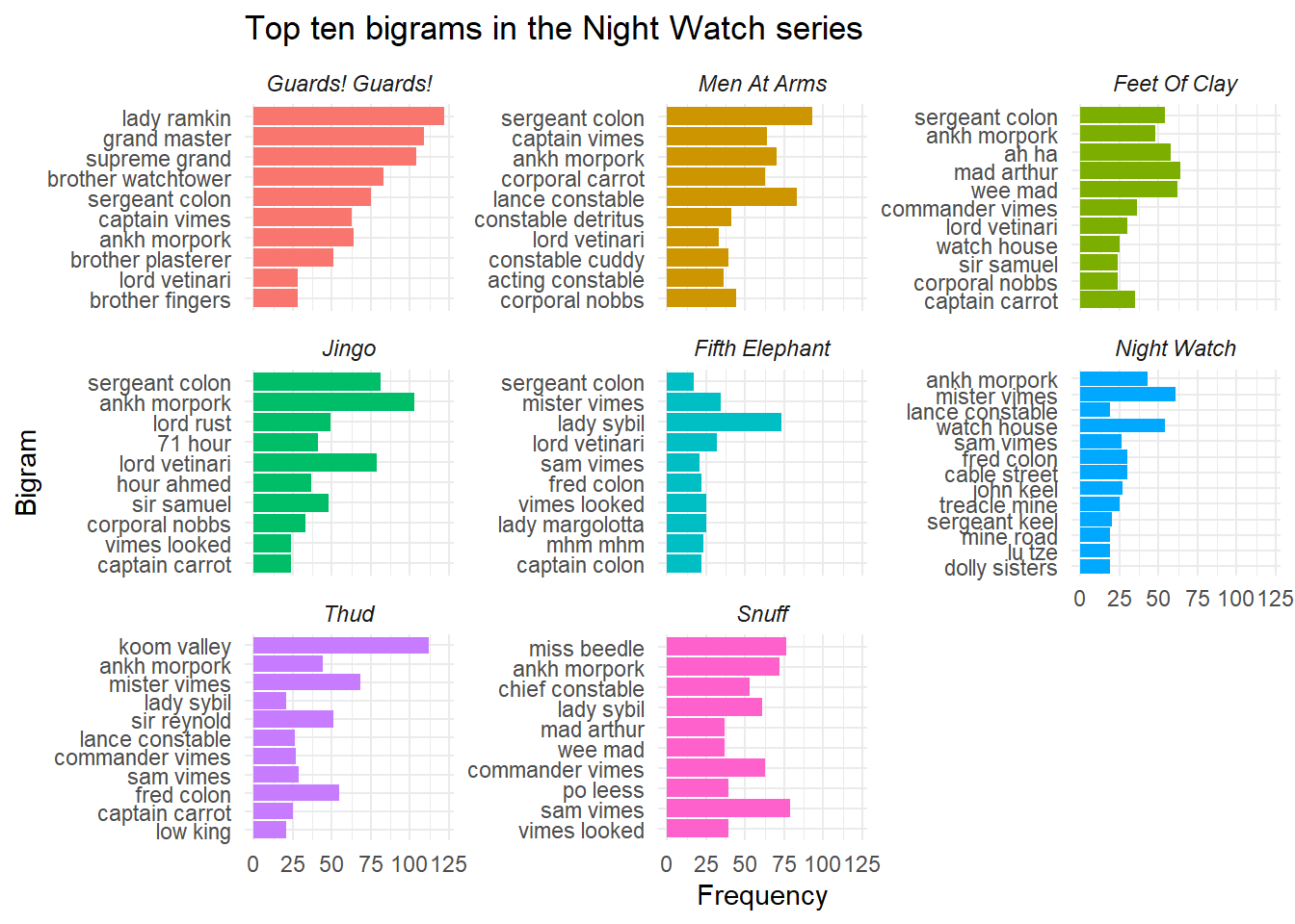
theme(panel.grid.minor = element_blank())## List of 1
## $ panel.grid.minor: list()
## ..- attr(*, "class")= chr [1:2] "element_blank" "element"
## - attr(*, "class")= chr [1:2] "theme" "gg"
## - attr(*, "complete")= logi FALSE
## - attr(*, "validate")= logi TRUEGendered_bigrams <- Watch_books %>%
unnest_tokens(bigram, sentence, token = "ngrams", n = 2) %>%
separate(bigram, c("word1", "word2"), sep = " ") %>%
filter(word1 %in% c("He", "he", "She", "she")) %>%
count(Book, word1, word2, sort = T) %>%
mutate(Grouping = case_when(word1 == "He" ~ "Male",
word1 == "he" ~ "Male",
word1 == "She" ~ "Female",
word1 == "she" ~ "Female"),
Grouping = factor(Grouping)) %>%
unite(Bigram, word1, word2, sep = " ") %>%
group_by(Book) %>%
top_n(10, n) %>%
arrange(Book, desc(n))
Gendered_bigrams %>%
ggplot(aes(x = reorder(Bigram,n), y = n, fill = Grouping)) +
geom_col() +
coord_flip() +
facet_wrap(~Book, nrow = 3, scales = "free_y") +
theme_minimal() +
labs(title = "Top ten Gendered bigrams in the Night Watch series",
x = "Bigram",
y = "Frequency") +
scale_color_brewer() +
theme(strip.text = element_text(face = "italic")) +
theme(panel.grid.minor = element_blank())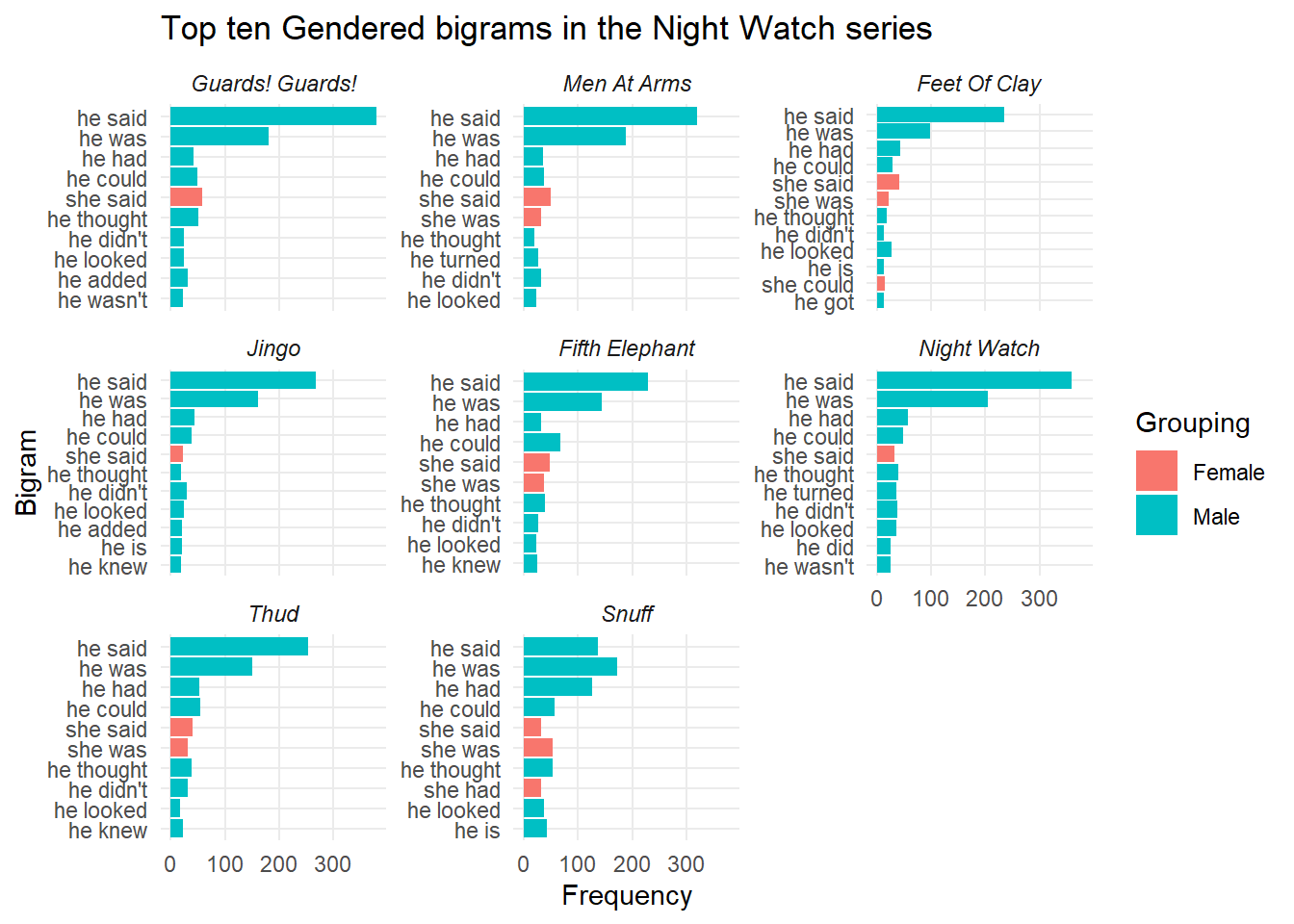
Moving on to inspirations from other areas, at the start I mentioned a text analysis based on ASOIAF, which also includes some neat dependency analysis using SPACY and the cleanNLP package via reticulate (though I had to do this on another laptop and import the data, I show the code here too). From this we can find the words most associated with specific characters, which can be used in conjunction with a term-frequency inverse document frequency analysis to find words strongly associated with a character that are less associated with other characters.
This showed a few key differences between main characters, such as Angua being associated with bounding, Nobby edging (usually away from danger) and Vimes thinking / realising (as he becomes a better detective).
use_python("/Library/Frameworks/Python.framework/Versions/3.7/bin/python3")

cnlp_init_spacy()

setwd("~/Desktop/Sam Vimes")

PDF_extraction_2 <- function(a){
  pdf_text(a) %>%
    paste(.,collapse = "")
}

WRD_extraction_2 <- function(x){
  readtext(x) %>%
    paste(.,collapse = "")
}

GG_2 <- WRD_extraction_2("D08 - Guards! Guards!.doc")


MAA_2 <- WRD_extraction_2("Men at arms.docx")


J_2 <- WRD_extraction_2("Jingo.docx")


GG_obj <- cnlp_annotate(GG_2, as_strings = TRUE)

MAA_obj <- cnlp_annotate(MAA_2, as_strings = TRUE)

J_obj <- cnlp_annotate(J_2, as_strings = TRUE)

Entities <- function(x){cnlp_get_entity(x) %>%
    filter(entity_type == "PERSON") %>%
    group_by(entity) %>%
    count %>%
    ungroup()%>%
    arrange(desc(n))}

GG_people <- Entities(GG_obj)

MAA_people <- Entities(MAA_obj)

J_people <- Entities(J_obj)

main_chars <- c("Carrot", "Nobby", "Angua", "Sergeant Colon", "Vimes", "Lady Ramkin", "Cuddy", "Gaspode")

dependencies_GG <- cnlp_get_dependency(GG_obj, get_token = TRUE)

dependencies_MAA <- cnlp_get_dependency(MAA_obj, get_token = TRUE)

dependencies_J <- cnlp_get_dependency(J_obj, get_token = TRUE)

full_dep <- bind_rows(dependencies_GG, dependencies_MAA, dependencies_J) %>%
  select(relation, word, word_target) %>%
  filter(word_target %in% main_chars & relation == 'nsubj' & word != "said") %>%
  group_by(word_target, word, relation) %>%
  count %>%
  arrange(desc(n))
full_dep <- read_csv("dependencies_DF.csv")
watch_tfidf <- bind_tf_idf(full_dep, word, word_target, n) %>%
group_by(word_target) %>%
top_n(10) %>%
arrange(word_target)
watch_tfidf %>%
ggplot(aes( x = reorder(word, tf_idf), y = tf_idf, fill = word_target)) +
geom_col(show.legend = F) +
theme_minimal() +
coord_flip() +
facet_wrap(~word_target, nrow = 3, scales = "free_y") +
labs(title = "TFIDF for charaters in Guards! Guards!, Men At Arms and Jingo!", x = "Word", y ="TFIDF")+
theme(axis.text.y.left = element_text(size = 6))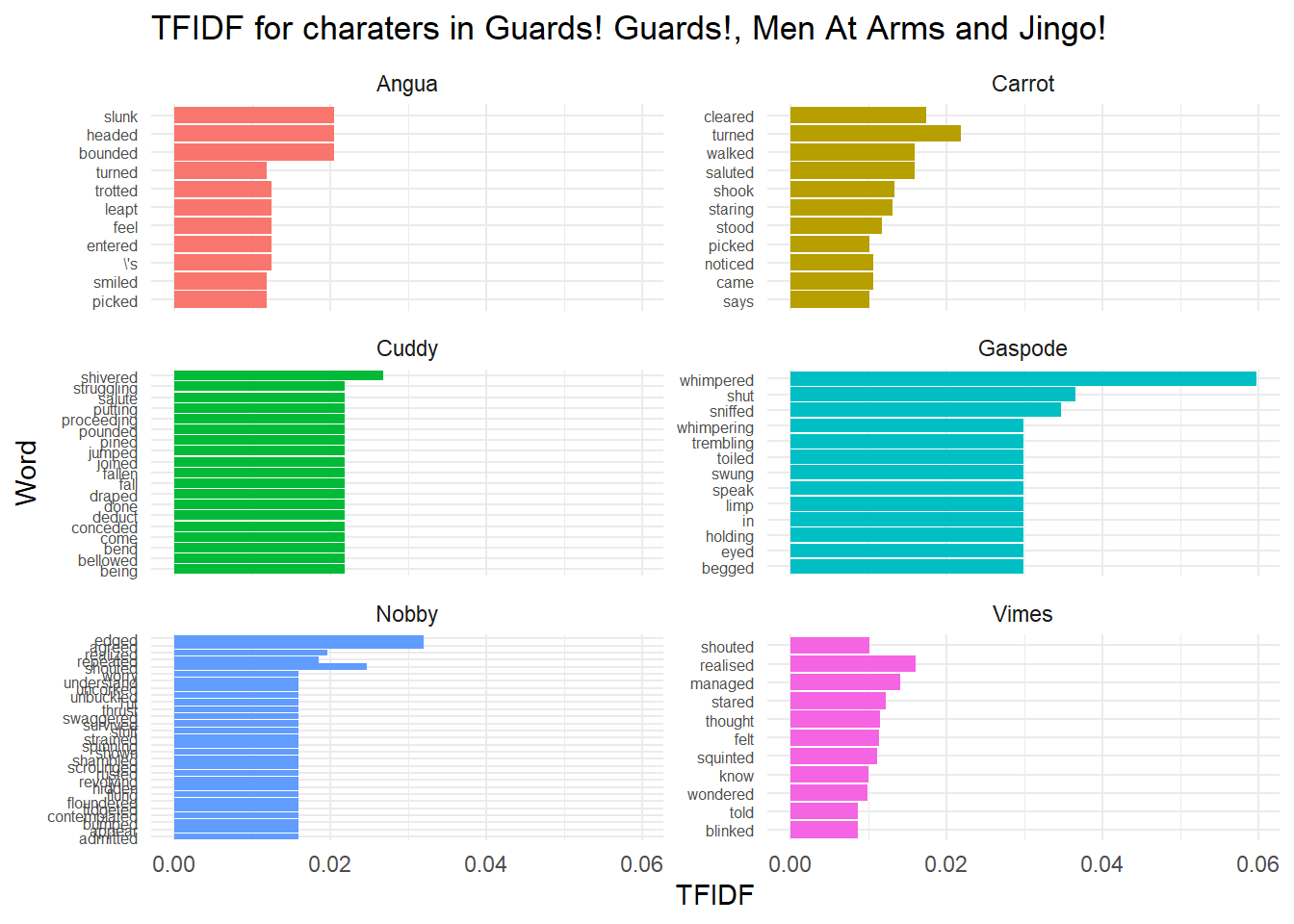
The final piece of analysis for this project was to perform subject topic modelling on the full series of books, aiming to divide them up into a number of related topics. This involved two different data prep approaches, the first being the conversion of the tokenised text into a document frequency matrix for modelling, and the second using the internal processing functions of the stm package to prepare the texts for a K search (in order to find an ideal number of topics). The two approaches were used due to some difficulty with using a dfm with the K search function. Once a suitable number of topics was chosen through the K search (6) the stm model was ran.
Watch_dfm <- Watch_books %>%
  unnest_tokens(word, sentence, token = "words") %>%
  anti_join(stop_words) %>%
  count(Book, word, sort = T) %>%
  cast_dfm(Book, word, n)


processed_books <- textProcessor(Watch_books$sentence, stem = F)

prepped_books <- prepDocuments(processed_books$documents, processed_books$vocab,lower.thresh = 5)

K_search<-searchK(prepped_books$documents,prepped_books$vocab,K=c(4:10))

plot(K_search)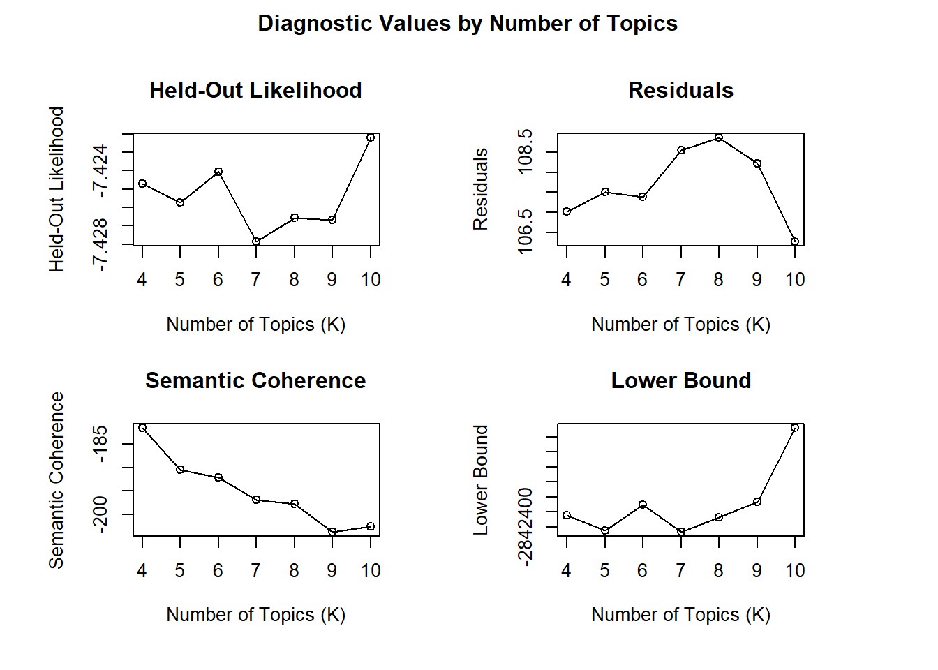
The outputs of this model could then be extracted from the model object, namely the top terms per topic (beta) and the distribution of books to topics (gamma). The terms graph of this data reveal that Vimes is fairly key for all except topic 2, and a number of terms were highlighted which indicate which book fits with each topic (IE the term carcer is included for topic 4, indicating this is likely fitted to the Night Watch book). The distribution graph shows that four books sit solely within one topic, whilst the other four books are spread between the two topics, two a piece. If I were to guess which these were I’d say Fifth Elephant and Thud fall into topic 1 (due to the dwarf and troll terms), leaving Jingo and Feet of Clay to fall into topic 6.
Watch_books_stm <- stm(Watch_dfm, K = 6, init.type = "Spectral", verbose = F)

tidy_stm <- tidy(Watch_books_stm)

top_beta <- tidy_stm %>%
  group_by(topic) %>%
  top_n(10, beta) %>%
  ungroup() %>%
  mutate(topic = paste0("Topic ", topic))

top_beta %>%
  ggplot(aes(x = term, y = beta, fill = as.factor(topic))) +
  geom_col(show.legend = F) +
  coord_flip() +
  facet_wrap(~topic, scales = "free_y", nrow = 2) +
  labs(title = "Top ten terms per theme of the Night Watch books", x = "Term", y = "Beta") +
  theme_minimal()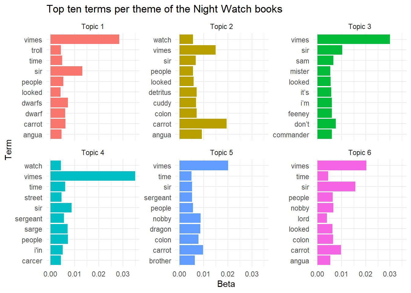
Watch_gamma <- tidy(Watch_books_stm, matrix = "gamma",
                    document_names = rownames(Watch_books_stm)) %>%
  mutate(topic = paste0("Topic ", topic))

Watch_gamma %>%
  ggplot(aes(gamma, fill = as.factor(topic))) +
  geom_histogram(show.legend = FALSE) +
  facet_wrap(~ topic, nrow = 2) +
  theme_minimal() +
  labs(title = "Document probabilities spread for each topic",
       y = "Number of books", x = "Gamma")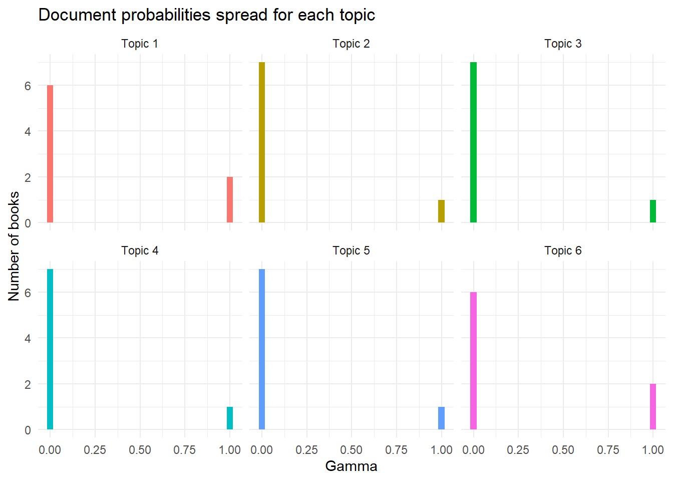
So, this brings me to the end of my analysis of the Night Watch books, using a few interesting techniques I’ve picked up from tutorials (mostly delivered by Julia Silge), hopefully you’ve enjoyed it!